In this project, I will employ several supervised algorithms to accurately model individual’s income using data collected from the 1994 U.S. Census. I will then choose the best candidate algorithm from preliminary results and further optimize this algorithm to best model the data. My goal with this implementation is to construct a model that accurately predicts whether an individual makes more than $50,000. This sort of task can arise in a non-profit setting, where organizations survive on donations. Understanding an individual’s income can help a non-profit better understand how large of a donation to request, or whether or not they should reach out to begin with. While it can be difficult to determine an individual’s general income bracket directly from public sources, we can (as we will see) infer this value from other publically available features.

The dataset for this project originates from the UCI Machine Learning Repository. The datset was donated by Ron Kohavi and Barry Becker, after being published in the article “Scaling Up the Accuracy of Naive-Bayes Classifiers: A Decision-Tree Hybrid”. You can find the article by Ron Kohavi online. The data we investigate here consists of small changes to the original dataset, such as removing the “fnlwgt” feature and records with missing or ill-formatted entries.

I had completed this project as part of my Data Science Nanodgree at Udacity. This project is implemented in a Jupyter notebook with Python code, and it is available on my GitHub.

Exploratory Data Analysis

Let’s have a look at the top row of our data set.

	age	workclass	education_level	education-num	marital-status	occupation	relationship	race	sex	capital-gain	capital-loss	hours-per-week	native-country	income
0	39	State-gov	Bachelors	13.0	Never-married	Adm-clerical	Not-in-family	White	Male	2174.0	0.0	40.0	United-States	<=50K

Note that the last column from this dataset, “income”, will be our target label (whether an individual makes more than, or at most, $50,000 annually.) All other columns are features about each individual in the census database.

A cursory investigation of the dataset will determine how many individuals fit into either group, and will tell us about the percentage of these individuals making more than $50,000.

Total number of records: 45,222

Individuals making more than $50,000: 11,208

Individuals making at most $50,000: 34,014

Percentage of individuals making more than $50,000: 24.78%

Featureset exploration

Now let’s have a look at each of the features in our dataset to ascertain their type, and range.

age: continuous.
workclass: Private, Self-emp-not-inc, Self-emp-inc, Federal-gov, Local-gov, State-gov, Without-pay, Never-worked.
education: Bachelors, Some-college, 11th, HS-grad, Prof-school, Assoc-acdm, Assoc-voc, 9th, 7th-8th, 12th, Masters, 1st-4th, 10th, Doctorate, 5th-6th, Preschool.
education-num: continuous.
marital-status: Married-civ-spouse, Divorced, Never-married, Separated, Widowed, Married-spouse-absent, Married-AF-spouse.
occupation: Tech-support, Craft-repair, Other-service, Sales, Exec-managerial, Prof-specialty, Handlers-cleaners, Machine-op-inspct, Adm-clerical, Farming-fishing, Transport-moving, Priv-house-serv, Protective-serv, Armed-Forces.
relationship: Wife, Own-child, Husband, Not-in-family, Other-relative, Unmarried.
race: Black, White, Asian-Pac-Islander, Amer-Indian-Eskimo, Other.
sex: Female, Male.
capital-gain: continuous.
capital-loss: continuous.
hours-per-week: continuous.
native-country: United-States, Cambodia, England, Puerto-Rico, Canada, Germany, Outlying-US(Guam-USVI-etc), India, Japan, Greece, South, China, Cuba, Iran, Honduras, Philippines, Italy, Poland, Jamaica, Vietnam, Mexico, Portugal, Ireland, France, Dominican-Republic, Laos, Ecuador, Taiwan, Haiti, Columbia, Hungary, Guatemala, Nicaragua, Scotland, Thailand, Yugoslavia, El-Salvador, Trinadad&Tobago, Peru, Hong, Holand-Netherlands.

Preparing the data

Before data can be used as input for machine learning algorithms, it often must be cleaned, formatted, and restructured — this is typically known as preprocessing. Fortunately, for this dataset, there are no invalid or missing entries we must deal with, however, there are some qualities about certain features that must be adjusted. This preprocessing can help tremendously with the outcome and predictive power of nearly all learning algorithms.

Transforming skewed continuous features

A dataset may sometimes contain at least one feature whose values tend to lie near a single number, but will also have a non-trivial number of vastly larger or smaller values than that single number. Algorithms can be sensitive to such distributions of values and can underperform if the range is not properly normalized. With the census dataset two features fit this description: “capital-gain” and “capital-loss.”

Skewed features in the dataset

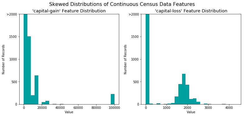
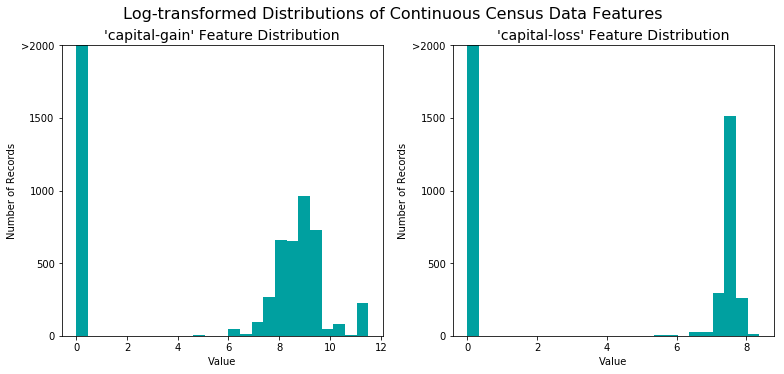
For highly-skewed feature distributions such as “capital-gain” and “capital-loss”, it is common practice to apply a logarithmic transformation on the data so that the very large and very small values do not negatively affect the performance of a learning algorithm. Using a logarithmic transformation significantly reduces the range of values caused by outliers.

The figure below shows the same features after log transformation was applied on the data. Note the range of values and how they are distributed.

Skewed features after log transform

Normalizing numerical features

In addition to performing transformations on features that are highly skewed, it is often good practice to perform some type of scaling on numerical features. Applying a scaling to the data does not change the shape of each feature’s distribution (such as “capital-gain” or “capital-loss” above); however, normalization ensures that each feature is treated equally when applying supervised learners. Note that once scaling is applied, observing the data in its raw form will no longer have the same original meaning. I have used sklearn.preprocessing.MinMaxScaler to perform this step.

Data preprocessing

During Exploratory Data Analysis, we saw there are several features for each record that are non-numeric. Typically, learning algorithms expect input to be numeric, which requires that non-numeric features (called categorical variables) be converted. One popular way to convert categorical variables is by using the one-hot encoding scheme. One-hot encoding creates a “dummy” variable for each possible category of each non-numeric feature.

Additionally, as with the non-numeric features, we need to convert the non-numeric target label, “income” to numerical values for the learning algorithm to work. Since there are only two possible categories for this label (“<=50K” and “>50K”), we can avoid using one-hot encoding and simply encode these two categories as “0” and “1”, respectively.

I used pandas.get_dummies() mehtod to perform one-hot encoding. After this step, we can see that the number of features have increased to 103.

Shuffle and split data

Now all categorical variables have been converted into numerical features, and all numerical features have been normalized. As always, we will now split the data (both features and their labels) into training and test sets. 80% of the data will be used for training and 20% for testing.

Evaluating model performance

In this section, we will investigate four different algorithms, and determine which is best at modeling the data. Three of these algorithms will be supervised learners , and the fourth algorithm is known as a naive predictor.

Metrics and the Naive Predictor

CharityML, equipped with their research, knows individuals that make more than $50,000 are most likely to donate to their charity. Because of this, CharityML is particularly interested in predicting who makes more than $50,000 accurately. It would seem that using accuracy as a metric for evaluating a particular model’s performance would be appropriate. Additionally, identifying someone that does not make more than $50,000 as someone who does would be detrimental to CharityML, since they are looking to find individuals willing to donate. Therefore, a model’s ability to precisely predict those that make more than $50,000 is more important than the model’s ability to recall those individuals. We can use F-beta score as a metric that considers both precision and recall:

$F_{\beta} = (1 + \beta^2) \cdot \frac{precision \cdot recall}{\left( \beta^2 \cdot precision \right) + recall}$

In particular, when beta = 0.5, more emphasis is placed on precision.

Looking at the distribution of classes (those who make at most $50,000, and those who make more), it’s clear most individuals do not make more than $50,000. This can greatly affect accuracy, since we could simply say “this person does not make more than $50,000” and generally be right, without ever looking at the data! Making such a statement would be called naive, since we have not considered any information to substantiate the claim. It is always important to consider the naive prediction for your data, to help establish a benchmark for whether a model is performing well. That been said, using that prediction would be pointless: If we predicted all people made less than $50,000, CharityML would identify no one as donors.

Supervised learning models

We can now select three of the supervised learning models that are appropriate for this problem that we will test on the census data.

Gaussian NB

This model is very good at classficiation of data that involves text, and therefore has found applications in SPAM detection, medical diagnosis that involves high recall models.

This model is a relatively simple model that handles large number of features well. It rarely overfits, and has a short model training and prediction times.

Gauissian Naive Bayes assumes the data follows a gaussian (normal) distribution, and may not work very well with data that does not follow this distribution. [1][2]

Since we are dealing with 10 plus features, I believe Gaussian NB could be a good fit for our problem The algorithm is simpler than the others, and might result in shorter model training, and testing times, which could be advantageous if it manages to get a good fbeta score.

Support Vector Machines (SVM)

SVM is widely used in text and hypertext configuration, and classification of images. It has also found applications in scientific community for the classification of proteins.

The biggest strength of SVM is that it not only helps with the classification problems, but also helps create a clear boundary among the sets through a configuralble hyper parameter C.

SVM does not work well when the sample data is not fully labelled. [3]

SVM might do well in our case since we are essentially dealing with a two class problem (income <= 50K and incomde > 50K) that requires a clear boundary.

Ada Boost

AdaBoost is a boosting algoirthm so it is naturally good at use cases that is suitable for its base estimator, which is typically a decision tree. It has applications in fraud detection in the insurance, and banking sectors. [4]

AdaBoost is an adaptive algorithm. Each weak learner is tweaked to handle the misclassifed points by previous weak learners. This inturn helps the algorithm to keep getting better and better with every iteration.

AdaBoost is sensitive to noise and outliers, which is it’s main disadvantage. [5]

AdaBoost typically uses a Decision Tree as it’s weak learner, and is often referred as the best out of the box classifer, which should work very well with our data.

Creating a training and predicting pipepline

To properly evaluate the performance of each model we’ve chosen, it’s important to create a training and predicting pipeline that quickly allows to effectively train models using various sizes of training data and perform predictions on the testing data. This pipeline was tested with 1%, 10%, and 100% of the training data to ascertain the model performance of our chosen algorithms. The results are given below.

Model performance

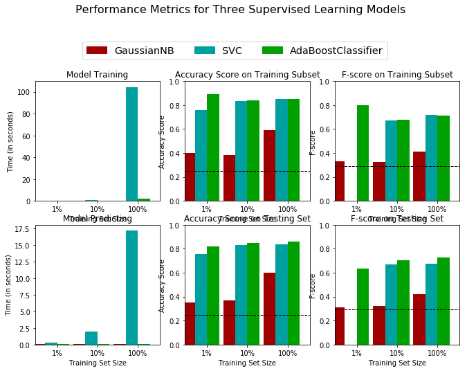
I have arrived at the conclusion that the AdaBoost Algorithm is the best candidate among the three algorithms chosen earlier. All three algorithms have fared better than the baseline, but SVC and AdaBoost performed the best, scoring between 0.6 to 0.8 in F-beta score. However, AdaBoost did have a slight advantage when we consider results from the testing data.

Moreover, the model training time for shot up exponentially (around 100 seconds on the training data and around 17 seconds for the testing data when 100% of the training data was used) for SVC algorithm, while it remained only around a few seconds for AdaBoost even when the entire training set was used. The algorithm is often referred to as the “best out of the box classifier”. These factors led to choosing AdaBoost algorithm.

Improving results

In this final section, I chose the best model, and performed a grid search optimization for the model over the entire training set (“X_train” and “y_train”) by tuning at least one parameter to improve upon the untuned model’s F-score. This is to identify by the optimum parameters for our chosen model. The results are given below.

Metric	Naive predictor	Unoptimized model	Optimized model
Accuracy Score	0.2478	0.8576	0.8605
F-beta score	0.2917	0.7246	0.7300

The optimized model had the accuracy score of 0.8605, and f-beta score of 0.7300. This is a slight imporvement over the unoptimized model.

The naive predictor had an accuracy score of 0.2478 and an fbeta score of 0.2917. Compared to this, the optimized model performs nearly 3.5 times better in accuracy and 2.5 times on f-beta score.