Linear regression is used to predict a continuous value. In this post we shall take a look at how Univariate Linear Regression - Linear Regression with one variable - works.
To better understand this concept, let us look at the example of predicting house prices. The table below is a training set with living area, and housing prices of a region. Our goal is to predict the price for a new house given its living area.
| Living area (sq. ft) | Price (1000s of Dollars) |
|---|---|
| (x) | (y) |
| 2104 | 460 |
| 1416 | 232 |
| 1534 | 315 |
| 852 | 178 |
| 3500 | 550 |
| 1700 | 315 |
| 500 | 125 |
| 2500 | 500 |
| 1900 | 400 |
| 750 | 150 |
| 200 | 250 |
| 800 | 200 |
| 700 | 400 |
| 500 | 350 |
| 800 | 250 |
| 50 | 150 |
| 2250 | 275 |
| 3200 | 475 |
| 2300 | 200 |
| 1000 | 190 |
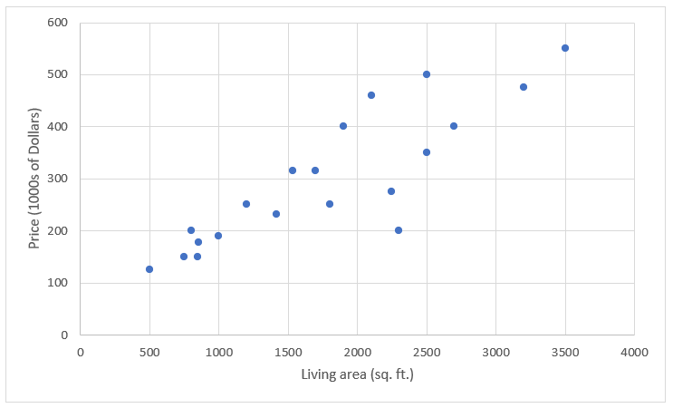
Now let us look a this data as a scatter plot to get a better idea about the data.

The scatter plot above gives us a good sense of the data. We can see that there is general trend where increase in living area corresponds to an increase in rental prices. There are exceptions ofcourse, but it seems to be the general trend.
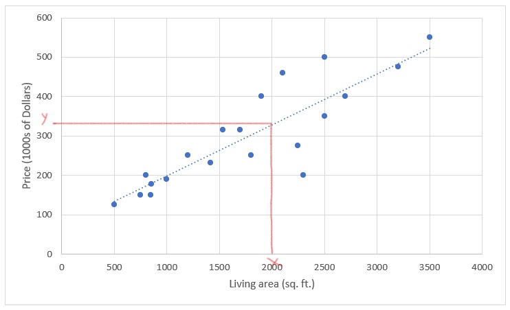
Now, if we can draw a straight line that fits very well with this data, we can use that to make predictions of the price. For a given living area on the x-axis, the corresponding intercept value on the y-axis from the straight line would give the prediction for its price.

The straight line here is an example for a linear function that works as our hypothesis, and hence the name Linear Regression. We call this Univariate Linear Regression as we are using only one variable - living area in this case - to make our predictions.
Equation of a straight line
A stright line is represented by the following equation:

where theta 0 is the y intercept, and theta 1 is the gradient, or the slope of the line. We can compute the slope using the following formula:

where (x1, y1) and (x2, y2) are two points on the line.
We can use these formulas to draw our straight line. But how do we draw it? There can be several values for theta, resulting in many possible lines through our data points. We need to pick some theta value that yields a line that provides the best fit for our data. This introduces us to the notion of a cost function, wherein we would assign a cost to each line with different theta values.
Cost Function
The cost function measures how well the line fits with the existing data points. There are many cost functions, but we shall use the Mean Squared Error function (MSE) here. This function takes the difference between predicted and actual values, squares it, and returns its average. In other words, the MSE function returns the average error across all the data points.

The line that gives us the smallest mean squared error, is the line with the best fit. This is nothing but finding the optimum values for theta that yields the line with the best fit.
Gradient Descent
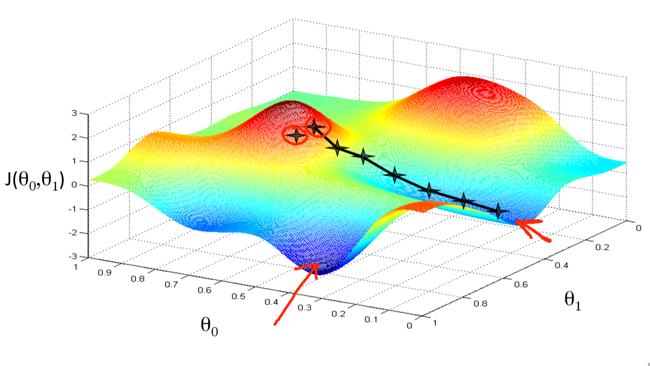
If we plot the values of theta 0 and theta 1 against the cost function J(theta 0, theta 1) as a 3D plot, we end up with a plot resembling hills and valleys. Starting out at a random point on top of this hill, we then need to descent the hill to arrive at a valley - known as a local minimum - that would correspond to optimum values for theta 0 and theta 1.

Gradient Descent Algorithm:
In order to descent the gradient descent hill, we need to apply changes to theta values in small increments. We can use the gradiet descent algorithm for this:
repeat untill convergence {

}
for theta = 0,1
When we substitue the cost function J with our MSE equation, we arrive at our final equation for theta 0 and theta 1.
repeat untill convergence {


}
where m is the size of the training set, xi and yi are individual values from the training set, alpha is the learning rate, and theta 0 and theta 1 are constant parameters that are updated simultaneously.
The alpha parameter is the learning rate that regulates the change to theta values. If it is too high, the changes become abrupt, and we might miss the local minimum. If it is too low, the gradient descent takes too long to converge. This method works well even when we keep the learning rate constant, as the partial derivative values comes close to zero as we approach the bottom of the valley.
Thus, by going through the gradient descent process, we end up with the optimum values for theta, which in turn gives us the best line of our hypothesis function. This method is called as batch gradient descent, as we go through the entire batch of data points before making adjustments to theta values.