Let’s face it, performing regression with one variable is just not that useful. Real world data involves tens, hundreds, or sometimes even thousands of features. We can scale up what we have learned in univariate linear regression to meet such needs.

Let us go back to our housing prices example. Imagine that we have more data to play with. Instead of just the square footage, we now have features, such as, number of bedrooms, number of bathrooms, neighbourhood data, length and breadth of the plot, etc.

We can write this in notational form:

m = number of training examples

n = number of features

x⁽ⁱ⁾ = features of the i^th training sample

x_j⁽ⁱ⁾= j^th feature in the i^th training sample

Putting all this together, our hypothesis function now becomes:

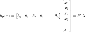
Vectorised form of the hypothesis

If we imagine x₀ as 1, we can represent the hypothesis its vectorized form:

Gradient Descent Algorithm

The algorithm remains largely unchanged, but now we need to account for the ‘n’ number of features.

repeat until convergence {

}

for j = 0..n

Feature Scaling & Mean Normalisation

It helps if all your features fall within in a set range. This is because gradient descent can easily converge on a small range, but takes more time to converge on a large range. It tends to oscillate back and forth down to the optimum when the values are uneven. So, our goal is to have all the values fall within a range, such as, -1 <= x <= 1. The most common methods employed for this purpose is feature scaling, and mean normalisation.

In Feature scaling, we modify all the features to fall within a set range. We can do this by dividing each feature by the range of the features, or its standard deviation. This results in a new range, or standard deviation of just one. In mean normalisation, we subtract the mean feature value from each of the features that results in a new mean value of zero. Often feature scaling and mean normalisation is applied together. This is known as standardisation, which can be expressed as:

Learning rate

To understand how learning rate works, we can plot the cost function, against the number of iterations of the gradient descent algorithm. In ideal conditions, the cost reduces with the number of iterations. We can repeat this process, and stop at a learning rate when we do not see a significant drop in cost after many iterations.

If the learning rate is high, gradient descent fails to converge as it may overshoot the local minimum. If it is too low, gradient descent takes too long to converge.

Feature Engineering

Selecting the right input features for the machine learning algorithm is very important. It is entirely possible to generate new features from existing features. For instance, we can combine lot length, and lot breadth into a single feature of lot area. We can even split a single feature into multiple features. For example, imagine that we are dealing with the sales figures of a sales team. In that case, a date feature can be split into day of month, week, quarter of the year, etc., if it helps with our analysis.

Polynomial Regression

There may be cases when a straight line is not going to neatly fit our data. In such cases, it would make much more sense to select a polynomial function as the hypothesis function. Feature scaling and mean normalisation becomes even more important in such cases, as we would be dealing with squares, and cubes of of feature values, i.e., very large numbers.